Four pieces of an automated inspection workflow — locating scans, finding features, fitting geometry, and deciding pass or fail — each implemented from scratch and run end to end. The figures and numbers below are the actual output of those runs.
How to read these. Everything here runs on simulated scan data with a stated noise model (15–20 µm RMS, outliers, scanner bias) and known ground truth — which means every accuracy claim is checked against truth by the code itself, not asserted by me. Real scanners add effects these simulations do not model, and each example says so plainly. I have no client case studies yet and will not invent any; this page shows the engineering. Code available on request.
01 · Scan registration
Eight partial scans, one coordinate frame — closed to 16 µm against ground truth
A scanner sees one side of a part at a time; software has to merge the views into a single model. Chaining scan-to-scan alignments accumulates error — drift — exactly the way dead-reckoning does. This pipeline registers eight overlapping partial scans of a machined part with robust ICP (iterative closest point, the standard cloud-to-cloud alignment method), measures 29 µm of accumulated drift where the chain closes on itself, and then corrects the whole chain at once by solving it as a pose graph — the same structure SLAM systems use.
321,445points, 8 scans
29 µmdrift at loop closure
24 → 16 µmmean map error after closure
9.6 stotal pipeline
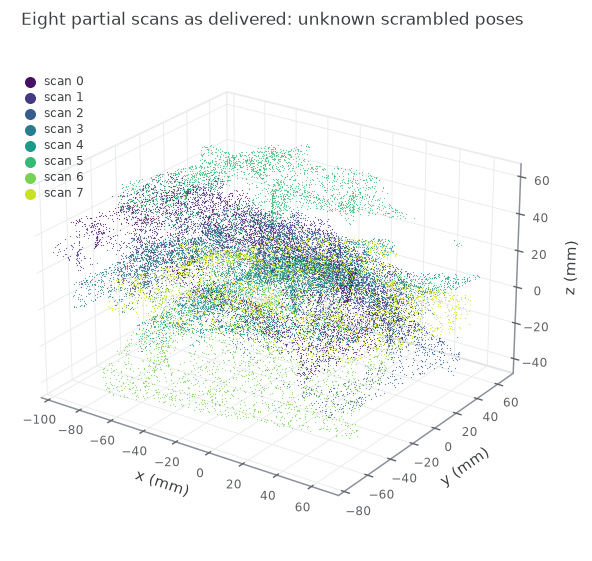
As delivered: eight partial scans, each in its own unknown pose — rotations of 10–21°, translations of tens of millimetres.
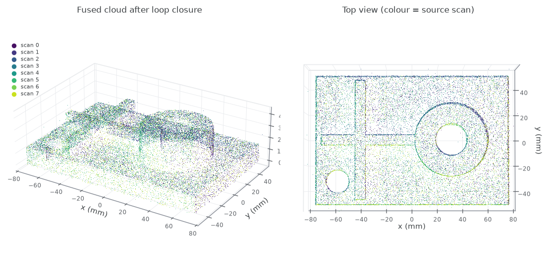
After registration and loop closure, coloured by source scan: bores, boss and ribs close cleanly across scan boundaries.
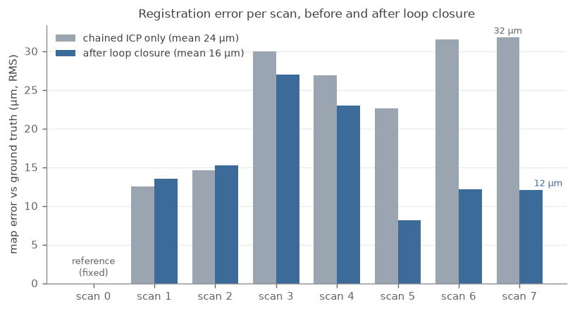
Per-scan error against ground-truth poses: sequential chaining drifts to 32 µm by the last scan; the pose-graph correction brings the chain end to 12 µm.What this does not show
Synthetic scans: real surfaces add shine, edge artifacts and reflections not modelled here.
Loop closure redistributes alignment drift; it cannot remove per-scan sensor bias, which sets the ~13–27 µm floor.
One geometry, one seed — a worked example, not a Monte-Carlo validation.
02 · Feature detection
Every hole on the plate found and measured, unattended
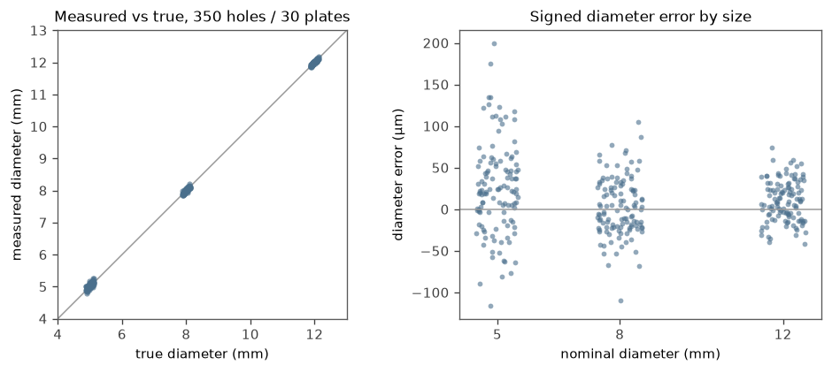
Point the software at a raw plate scan and it finds the holes itself: fit the plate plane robustly, find the data voids, trace each hole's boundary loop, fit a circle to it. No clicking, no per-part programming, no template that breaks when a hole moves. Across 30 simulated plates with randomized hole patterns — including plates with missing and off-pattern holes — it found 350 of 350 with zero false positives, and wrote an operator-style measurement table for each plate.
350 / 350holes detected, 30 plates
0false positives
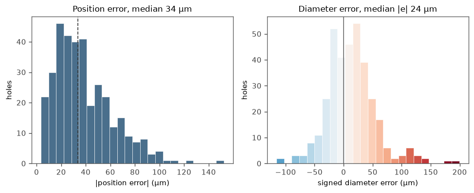
34 µmmedian position error
0.18 sper plate (~170k points)
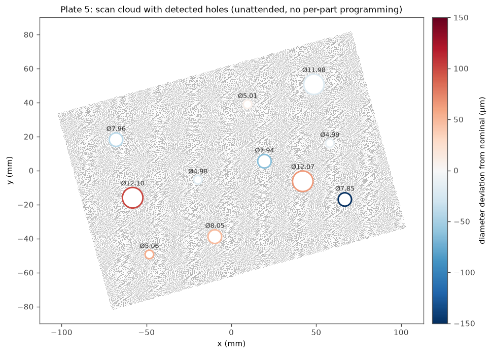
One plate: every hole detected and measured unattended; ring colour is diameter deviation from nominal, annotation is the measured diameter.
Measured vs true diameter for all 350 holes; median absolute diameter error 24 µm at 18 µm scan noise.
Error distributions across the batch: position (median 34 µm) and signed diameter error.What this does not show
This scenario did not stress the detector to failure — holes of 5 mm and up at this point density are comfortably detectable. Smaller holes, sparser scans or edge-adjacent holes would be harder.
Diameters carry a small positive bias (+13 µm mean) from the chamfer-edge model; a real system adds calibration on top.
Coordinates are plate-plane coordinates — no datum alignment or true-position evaluation here (see example 04 for that).
03 · Robust geometric fitting
Fitting that survives contaminated data
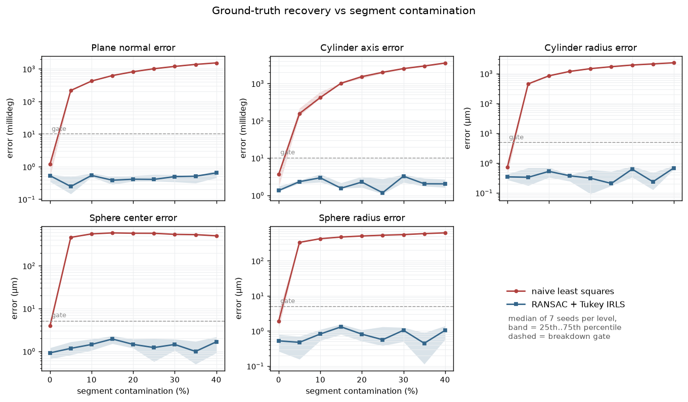
Every measured feature ends as a geometric fit — a plane, cylinder or sphere computed from points. The textbook fit assumes every point belongs to the feature. Real segments are contaminated: clamp faces, neighbouring surfaces, spray. On scans with 17 µm noise and known ground truth, plain least squares is already off by whole millimetres of radius at 5% contamination — while producing a number that looks perfectly plausible. The robust pipeline (RANSAC consensus selection, then Tukey-weighted refinement) recovers radii to about 1 µm with 40% of the segment contaminated.
5%contamination breaks naive LSQ
40%robust pipeline still ~1 µm radius
1,930 µm vs 0.6 µmradius error at 30%, naive vs robust
6.3 s1,000,000-point cylinder fit
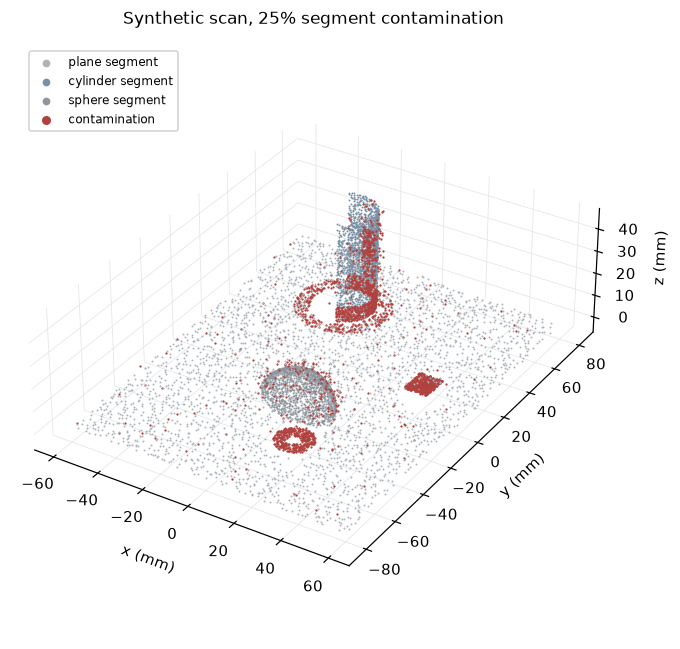
The test scene at 25% contamination: red points — clamp faces, adjacent-surface leaks, spray — sit in the feature's segment but do not belong to it.
Ground-truth recovery vs contamination, five metrics, median of seven seeds: naive least squares crosses every breakdown gate at the first non-zero level; RANSAC + Tukey stays flat to 40%.
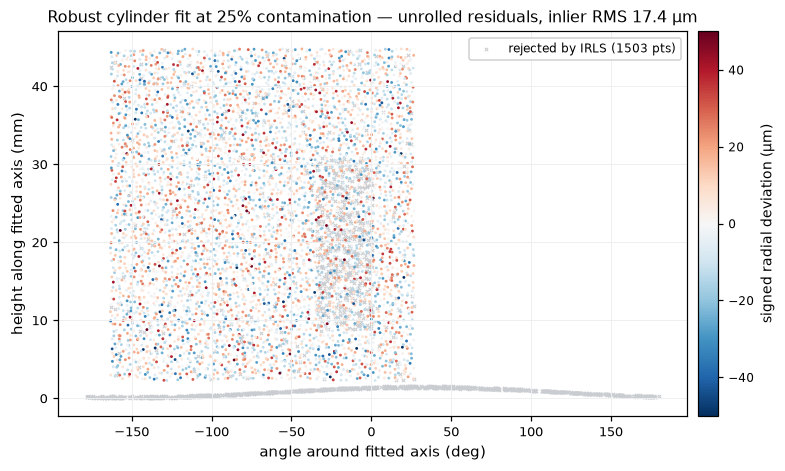
The robust cylinder fit's unrolled residual map: inliers show the 17 µm noise field; the rejected clamp strip appears as excluded clusters.What this does not show
Contamination here is structured but favourable to consensus methods; a near-coaxial mimicking feature could defeat RANSAC and is not exercised.
Thresholds assume the known noise level; on a real instrument they must be qualified from measured residuals.
Real scanner artifacts — waviness, density variation, systematic bias — are not modelled in this example.
04 · Unattended batch inspection
Twenty-five parts, arbitrary poses, zero clicks: locate, build the datum frame, decide
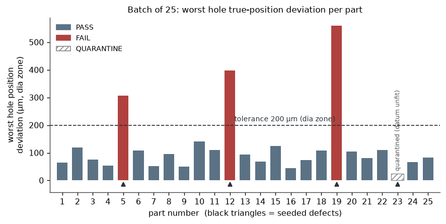
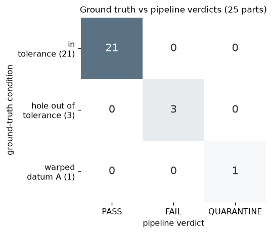
The capstone: everything above in one pipeline. Twenty-five parts of one family arrive in random orientations. For each, the software segments the faces, fits the three datum planes, and constructs the A|B|C datum reference frame exactly as a metrologist would — primary levels, secondary orients, tertiary stops — then evaluates six hole positions against a Ø0.2 mm position tolerance in that frame. Four parts carried seeded defects. All four were caught with the correct failure mode, with zero false alarms — and the one part whose primary datum face was warped was quarantined as un-evaluable rather than guessed at, because a datum frame built on a bad fit produces confident nonsense.
4 / 4seeded defects caught
0false alarms
1part quarantined, not guessed
0.39 sper part · 153 parts/min
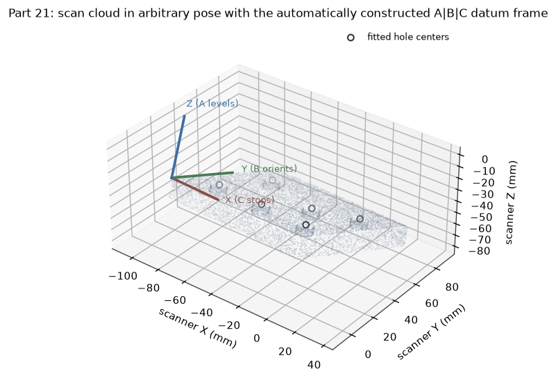
One part as scanned, in an arbitrary pose: the A|B|C datum frame triad constructed automatically from fitted faces, with the six fitted hole centers.
The batch at a glance: worst hole position deviation per part against the 200 µm tolerance; failures red, the quarantined part hatched.
Ground truth vs pipeline verdict for all 25 parts: exactly diagonal — every good part passed, every defect caught, the bad-datum part quarantined.What this does not show
The pipeline assumes the datum faces and bores are captured — a planned scan of a known part family, not an unknown part.
Quarantine thresholds were set with knowledge of the simulated noise; a production cell qualifies them against gauge studies.
Hole centers use a projected circle fit with the axis normal to datum A; tilted or tapered bores need a full cylinder fit.
Where this fits in your shop
These four pieces are the algorithm layer of inspection automation. In production they live inside your platform's scripting environment — I specialise in ZEISS INSPECT — or alongside it as external tooling that feeds your quality system. The part is yours, the method is yours and stays approved by your metrology owner; what I bring is the software engineering that makes it run unattended, at rate, with numbers you can defend.
If you have a workflow that should run without someone standing over it, hello@metrologymaven.io — one workflow and one sentence about where it hurts is the ideal first message.